
Methods
Hybrid Solver
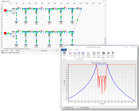
In order to apply a hybrid solver technique, the complex microwave system needs to be subdivided into smaller subsystems or components. Each subsystem or component will then be solved for RF
parameters at its interfaces with a method best suited for the task.
Each solver operates within its comfort zone without reaching limitations requiring the user to stop the software execution and manually interfere with settings or options. Improved accuracy as
convergence goals shift from assembly level to component level where they can be more easily controlled. There is no need for meshing connecting waveguides due to application of transmission line
equations describing multi modal wave propagation inside structures of uniform cross section.
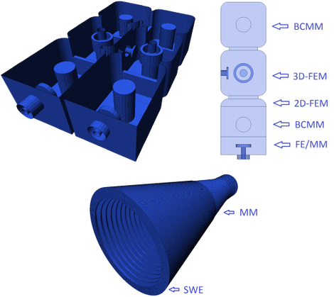
MM = Mode Matching
FE = Finite Element Method (FEM)
BCMM = Boundary Contour MM
SWE = Spherical Wave Expansion
PO = Physical Optics for reflectors
Mode Matching
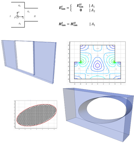
Mode-Matching (MM) method and derivations: The electro-magnetic fields inside the structure under consideration are expanded into known, analytic solutions of Maxwell's equations for similar
geometries. The boundary conditions are fulfilled using a Galerkin procedure on the element surface. Usually only a few of these (some 100) analytic solutions (modes) are needed for
sufficient convergence of the results, so this method is very fast and has low computational requirements. Because, there are only few structures with known, analytic solutions of Maxwell's
equations (e.g. rectangular + circular cavities + waveguides), this method is applicable only to certain geometries and thus lacks some geometric modeling capabilities.
On the other side the derivation from pure mode matching to 2D Finite Element Method (2D-FEM) Mode-Matching as well planar 2D-FEM Mode-Matching broadens the application range by multiple. In such
case the 2D-FEM mesh determines the eigenvalue of an arbitrarily shaped contour.
The Boundary-Contour-Mode-Matching (BCMM) method is another derivation of the pure mode matching code. BCMM supports the fast and accurate computation of shaped cavities, even with partial height
and dielectric posts.
In case of antennas the spherical wave expansion / mode matching method leads to short computation times for horn antennas in particular for the radiation from a circular aperture. The
computation of reflectors is an alternating process between Spherical Wave Expansion (SWE) and Physical Optics (PO).
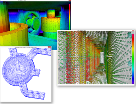
3D-FEM
Based on the 3D Finite Element Method (3D-FEM) with base function up to 3rd order, µWave
Wizard™ supports the analysis and optimization of elements with complex geometries that are not suitable for the Mode-Matching method. These are user defined
elements from the modeler library elements i.e. screws or probes penetrating into cavities, draft angles for die-casting technique and smooth wall profiled tapers. The modal absorbing boundary
conditions at the element ports ensure full multi-modal compatibility and interchangeability with all other MM-, BCMM- and 2D FEM-elements at the S-parameter level. Lossy and anisotropic
materials, such as ferrites, are fully supported. Creation of the element surfaces and the tetrahedral volume meshes is fully automated, including automated local mesh refinement around critical
geometries. User-supplied geometries can be imported from CAD files
(STL/STEP/IGES).
3D-FEM - Mesh Morphing
(New in µWave Wizard™ 2020)
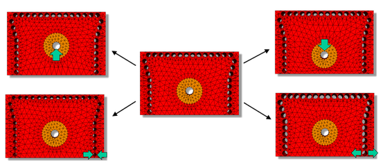
Mesh morphing is a new feature introduced in version µWave Wizard™ 2020 to accelerate
optimizations of complex structures using the 3D FEM method. The mesh topology is kept constant as long as possible, instead the mesh nodes are moved as dimensions change. In this way the "noise" introduced by mesh generation is ignificantly reduced, which improves the convergence of radient type optimizers, like the "Extrem" or "Powell" optimizers. The convergence behaviour of gradient type optimizers is comparable to pure MM elements, even when a very coarse discretization is used. The computation is also faster, since the mesh generation is done only at beginning of the optimization and the set-up time for mesh morphing is not longer than a single mesh generation.
This feature supports all kinds of dimension changes: tuning screw depths and diameters, tap positions, case, iris and cavity dimensions, bend and draft angles, milling radii, ridge widths and use defined equations, etc. are supported. The dependency of mesh node positions on the optimization variables is detected fully automatically. The only user interaction required to take advantage of mesh morphing is to "swich on" this feature.
Mesh morphing is available for all kinds of parametrized 3D FEM based elements, including user-defined modeler elements, as well as 3D FEM simulations on circuit level. Typical use cases of mesh morphing are the creation of complex filter designs from scratch with "real" 3D dimensions and the fast performance of feasibility studies. Starting with a coarse discretization and low order FEM base functions, the high speed 3D FEM optimization quickly leads to an initial structure design with dimensions close to the final design goal. In order to achieve the final specifications, the structure is fine-tuned with higher levels of accuracy, which only requires a few iterations due to the good starting values.
Lumped Elements
µWave Wizard™ contains a library which supports lumped element designs. There are low-level elements for user-defined
RLC-networks as well as ‘ideal filter’ elements representing an entire filter given by type (low-pass, band-pass, etc.), degree (number of resonators) and topology (coupling matrix). These
elements are especially useful for an easy setup and fast pre-optimization of complex structures (e.g. multiplexers) by equivalent networks. A lumped element circuit or an “ideal filter” element
can be connected to waveguide components or waveguide circuits in form of a sub circuit, using only fundamental mode connection. This is a convenient approach for optimizing complex structures
where waveguide components and lumped element circuits representing different kinds of filters are combined for initial optimization and feasibility studies. Throughout the subsequent
design/optimization process, one lumped element circuit at a time will be replaced by a real waveguide filter with matching electrical performance until the final design consists of waveguide
filters only.
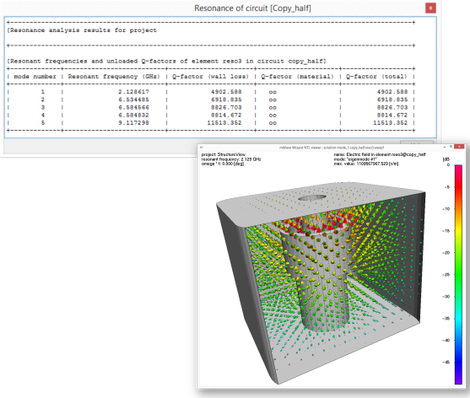
Resonance Analysis
The computation and optimization of resonant frequencies is of particular importance in the process of designing filters, especially in the design of combline and dielectric resonator
filters. µWave
Wizard's™ 3D-FEM solver offers the opportunity to determine and optimize the resonant frequency of almost any structure. Besides computing resonant frequencies, the resonance
analysis tool also simulates the electromagnetic fields within the resonator and computes the resonator's Q-factor. Using µWave
Wizard's™ 3D-viewer, the resonance analysis tool supports visualization and plotting of electromagnetic fields of resonant modes.
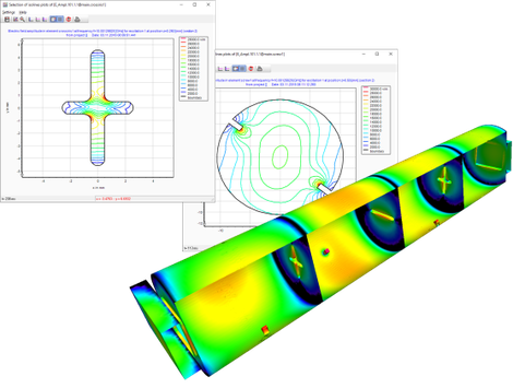
Field computation and visualization
The field computation feature of the µWave Wizard™ is suited for the visualization of the electric and magnetic fields at
critical parts inside waveguide circuits and structures. From the output of the field plots the user can estimate the power handling capabilities of filters and transitions and thus eases the CAD
of high-power microwave devices. For the field calculation inside a 3D-FEM element or a 3D-FEM computed circuit most settings and its handling are the same as for the "normal" field
calculation with MM/BCMM and 2D-FEM. The main difference is, that 3D vector plots of the fields are generated for the whole volume of the structure instead of plots along certain planes inside
the element. Furthermore the solutions can be exported to animate the propagation of the field (E, H, S) as a scalar of vector plot. This eature is very useful to get a feeling for the
EM-model.
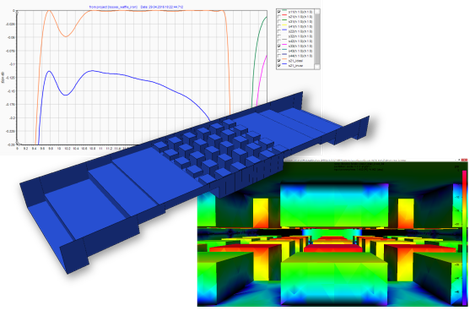
Losses
The 3D-FEM solver supports rigorous inclusion of losses. Losses, either dielectric or caused by finite surface conductivity, are an integral part of the calculation. In addition, surface losses
in planar structures, step discontinuities or any other structure that can be solved by using Mode Matching, 2D-FEM and BCMM, can be taken into account using a perturbation method at almost no
additional computational effort by not requiring a 3D-FEM solver.
Radiation
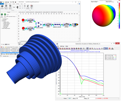
This feature supports computation and optimization of far and near field patterns of radiating elements. The patterns are computed with single mode excitation into the circuit, for an arbitrary number of frequency points at an arbitrary port. The excited mode can be selected from the variety of all accessible modes at the respective ports. This enables the design and optimization of complex multi-port feed networks and simultaneous optimization on telecom and tracking mode patterns. The field patterns are derived from spherical wave coefficients of the radiating element at a fixed radius. This method guarantees very fast computation of a radiating element and provides the pattern as typical 2D and 2D-isoline plots as well a complete 3D plot. The spherical wave expansion coefficients are also used by µWave Wizard™ for simulating reflector antennas and can be exported in ASCII file format as an input for other reflector antenna tools. The radiation element is typically connected directly to a circular horn or to a circular waveguide. Depending on the upstream network the radiation element even supports cluster feeds, patch antennas and slot arrays with a moderate number of slots, depending on the radius of the waveguide aperture. Pre-defined performance parameters such as max-gain, aperture efficiency, 3dB beam width, phase center location, edge taper etc. simplify setting up an antenna analysis or optimization.
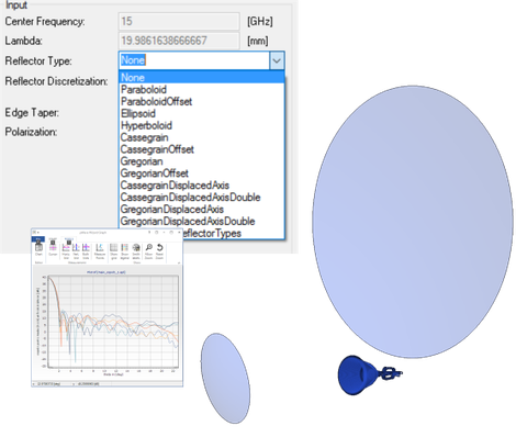
Reflector
The radiation from a rationally symmetrical reflector is an enhancement of the radiation-element. The radiation of the horn-antenna is used as a feed-system for standard reflector-types. From the
spherical-wave-coefficients the surface-current-density is calculated on the reflector using the physical-optics (PO) approximation. The surface-current-density is then expanded into
spherical-waves-coefficients again. These coefficients are used to calculate the far field radiation of the reflector, and can also be used as a feed-system to another reflector, as well, to
calculate a double reflector antenna. Beside the visualization of the pattern the surface current density on the reflector can be shown with the µWave Wizard™ 3D-viewer. All type of reflectors including the feeding network can be optimized on the typical antenna performance
parameters.